Monitoring and retraining strategies for demand forecasting models

Demand forecasting is one of the most impactful machine learning projects in many industries. And one of the most challenging ones too: the models are entangled with business processes that drive decision-making.

To illustrate this, let’s consider a scenario of a supermarket chain with dozens of stores across the country. This company has a demand forecasting model that runs weekly to estimate the number of products for each product category they will sell.

The executive team then uses this model’s outputs to guide strategic development. The supply chain team relies on the model to ensure they can fulfill all projected orders. The marketing team frequently gets involved in a downstream process, where they use the model’s projections to launch promotions and other marketing efforts to incentivize the rotation of products.

If a model like this is left alone, it might cause significant harm to the entire operation. With consumer trends evolving over time, the model’s performance will probably deteriorate.

That is why it becomes crucial to retrain the model on time and constantly monitor its performance. This way, model maintainers who worry about the model’s performance (a.k.a data scientists and ML engineers) should get notified when something is not looking right and get their hands on the issue as soon as possible before the “bad” predictions affect the executive, supply, and marketing teams.

Demand forecasting monitoring challenges

Delayed ground truth

Probably the biggest challenge in monitoring forecasting models is that we often don’t realize the model’s predictions are incorrect until they have already misled us.

In the case of the demand forecast for a supermarket chain, we monitor MAE (Mean Absolute Error) per product category. To assess MAE, we need to wait for a week due to a delay in the feedback loop. This poses a significant risk to the core business operations.

A way to address this issue is to apply performance estimation techniques. Estimating performance can feel like a superpower. We no longer need to wait for the ground truth to have visibility on how an ML model is performing with production data. In the case of demand forecasting, we can use DLE (Direct Loss Estimation) to estimate the MAE metric with any frequency that we want. You can’t predict the errors of your model… Or can you? article gives a great explanation of how DLE works.

If ground truth becomes available at the end of every week, we could monitor the estimated performance on a daily basis and calculate the realized performance every week. This would give us a more accurate view of the model’s performance over time.

The multi-model problem

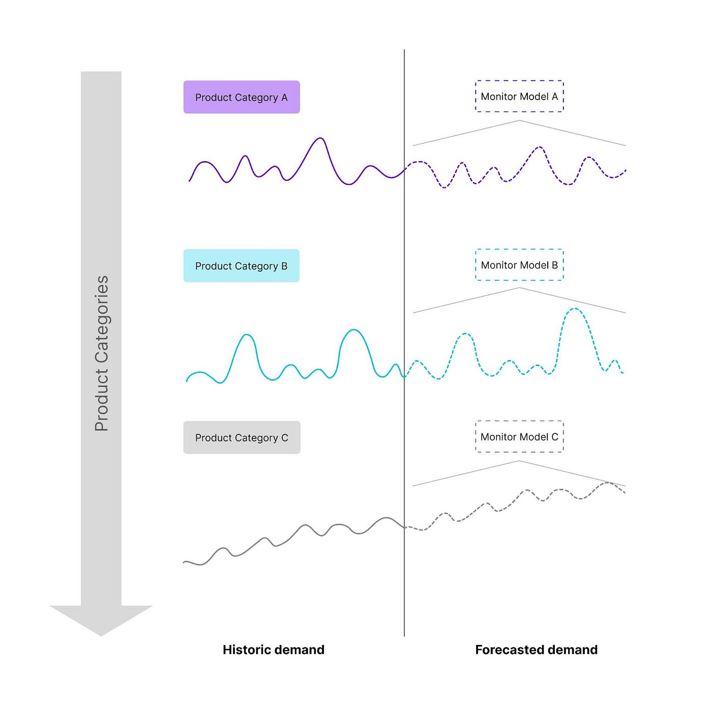
Demand forecasting often involves predicting demand for not only one product but the demand for several products of a company’s product portfolio, which means building a different model for each product or product category. We are talking about hundreds or even thousands of models.

Monitoring this type of architecture can easily get out of our hands. A way to address this problem is by leveraging the performance thresholds of each product category individually. It makes sense since the business impact of bad prediction varies per product. In the case of a supermarket, ordering too many ice creams would not be as bad as ordering too many bananas.

So in the event of a performance drop that can not be corrected with a simple retraining on a new dataset, we can temporarily quarantine the specific model, look for the issues, retrain the model (new data selection, hyperparameters, new features, new type of model) and put it back into production only if the new model shows improved performance on a test set vs the old model.

Monitoring building blocks

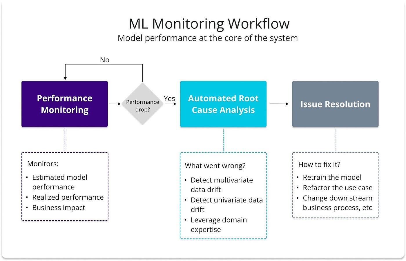
Model monitoring should be performance-centric. What that means is that we will obsess over performance, estimated and realized performance. If a performance drop is observed we perform a root cause analysis to find what went wrong and later resolve the issue by retraining the models with the right data.

The following diagram shows a high-level overview of a performance-centric monitoring workflow. It consists of three main building blocks: Performance Monitoring, Automated Root Cause Analysis, and Issue Resolution.

Performance monitoring answers the question: are my models still performing well? By focusing on monitoring three main metrics:

• estimated performance

• realized performance

• business value

Estimated performance can be calculated when ground truth is not known yet using the DLE algorithm mentioned earlier. It can be compared to the realized performance when the ground truth becomes available.

Also, whenever it is possible to translate those model performance metrics into business values it is advised to also monitor them at the top level of the monitoring workflow. Measuring the model’s performance in terms of MAE/RMSE/etc is great but it is always more impactful if we can quantify that in terms of $.

In the eventuality of a drop in performance, an automated RCA (Root Cause Analysis) can help answer: what went wrong? The RCA block uses multivariate and univariate drift detection methods, data quality checks, and concept shift detection methods to help data scientists investigate the underlying cause of the model degradation. NannyML’s article about the new way to monitor ML models explains RCA in more detail.

Once we have found the underlying cause of the performance issue, we can search for the best technique to fix the problem. The appropriate solution is context-dependent, there is no simple issue resolution for every problem. For demand forecasting models, if the issue was not caused by data quality problems or a heavy concept shift, gathering the latest data and retraining the models is usually the go-to solution.

Orchestration of model monitoring and intelligent retraining

In the previous article about batch processing, we discussed how demand forecast model orchestration logic is defined when you need 5 models for different product categories. In that example, the modes are retrained weekly (a full week of data is required), and predictions are generated daily.

Retraining weekly might not be necessary, so we suggest intelligent retraining. Here we estimate MAE (mean absolute error) using the “nanny model” (DLE that estimates the errors of the core model) and only retrain when the estimated MAE goes below the threshold. In that case, the process would look as follows:

The nanny model does not have to be retrained every time we retrain the model. It is only needed in case of big changes in the core model (different algorithms, different features, significant data drift).

The same workflow can be used to generate data for the demand forecasting monitoring dashboard. The monitoring dashboard would contain the daily predictions per product category, daily estimated MAE, and weekly realized MAE with associated business value.

Benefits of intelligent retraining

Automated retraining is the industry’s go-to solution to prevent model performance degradation. A fixed schedule or retraining based on shifts in feature distributions (univariate drift) are common practices. Orchestrating a retraining process based on data drift might not yield the best results, as not every feature drift necessarily leads to a drop in performance. So, what are the benefits of intelligent retraining compared to the fixed schedule?

Decrease cloud costs (retrain only models that need it)

With a fixed schedule, we might sometimes be retraining models that don’t need to be retrained yet. An intelligent schedule would alleviate cloud costs, as only models with an estimated performance drop would be retrained.

Following the supermarket scenario with a multi-model approach (one model per product category), let’s assume we have 50 product categories, and one model for each category. If we stick to a fixed schedule with a weekly period, that would result in 2600 retraining processes per year.

On the other hand, we could significantly reduce retraining expenses by leveraging the performance thresholds of each product category individually. In the event of a performance drop, we can then apply the retraining pipeline to that specific category only.

Decrease time to deploy (parallel retraining of fewer models)

Similar to before, by reducing the number of retraining updates, we are able to decrease the overall amount of time spent deploying those updated models. Let’s say that in a week only 10 product category models experienced a decrease in performance. This would trigger the intelligent schedule to retrain and deploy only those 10 models, as opposed to the 50 we would have under a fixed schedule.

To sum up

In summary, effective monitoring and retraining strategies are fundamental for maintaining the performance of demand forecasting models, especially in complex operational environments, as demonstrated in our supermarket chain example. Following a performance-centric monitoring approach allows us to have observability of model performance even in the absence of ground truth.

Are you hungry for code?

In our next blog post, we will take these ideas and implement a practical monitoring scenario using a real-world dataset. Stay tuned!