

Databricks recently introduced Free Edition, which opened the door for us to create a free hands-on course on MLOps with Databricks.
This article is part of that course series, where we walk through the tools, patterns, and best practices for building and deploying machine learning workflows on Databricks.
In this lecture, we’ll dive into one of the most critical (and often misunderstood) aspects of production ML: monitoring.
Watch the lecture on Youtube:
In a ML system, you need to monitor metrics that go beyond the ones you’d expect in any production system (such as system health, errors, and latency, KPIs and infrastructure costs).
In classic software, if code, data, and environment stay the same, so does behavior. ML systems are different: model performance can degrade even if nothing changes in your code or infra because ML is driven by the statistical properties of your data. User behavior can shift, seasonality or upstream data can change.
All can cause your model to underperform, even if everything else is “the same.” That’s why MLOps monitoring includes data drift, model drift, and statistical health, not just system metrics.
Data Drift: It happens when the distribution of the input data shifts over time, even if the relationship between inputs and outputs stays the same. For example, let’s say there is a lot of new houses entering the market in a certain district. People’s preferences, the relationship between features and price stays the same.
But because the model hasn’t seen enough examples of new houses, its performance drops, not because the logic changed, but because the data shifted. In this case, data drift is the root cause of model degradation.
Concept Drift: It happens when the relationship between input features and the target variable changes over time so model’s original assumptions about how inputs relate to outputs no longer holds. Let’s look at housing prices example: new houses enter the market, and the government introduces a subsidy for families with children which leads to larger houses sold for lower prices. This is a shift in the underlying relationship between features like house size and the final price. Even if the input data distribution doesn’t change much, the model’s predictions will become less accurate
Not all drift is bad! Sometimes, your model is robust to input changes, and performance remains stable. Check this article for a real example. Suppose you detect significant data drift in the “temperature” feature using Jensen-Shannon distance. But, when you check the model’s MAE (Mean Absolute Error), performance is still well within acceptable bounds. The main point is that not all drift requires action, so we need to monitor both data and performance before retraining or raising alarms.
Let’s dive into what Databricks has to offer for ML monitoring.
ML Monitoring in Databricks
Databricks Lakehouse Monitoring lets you monitor the statistical properties and quality of the data in your delta tables. We can also use it to track the performance of machine learning models and model serving endpoints by creating inference tables with model inputs and predictions.
Databricks automatically generates a few key components to help you track model and data health.
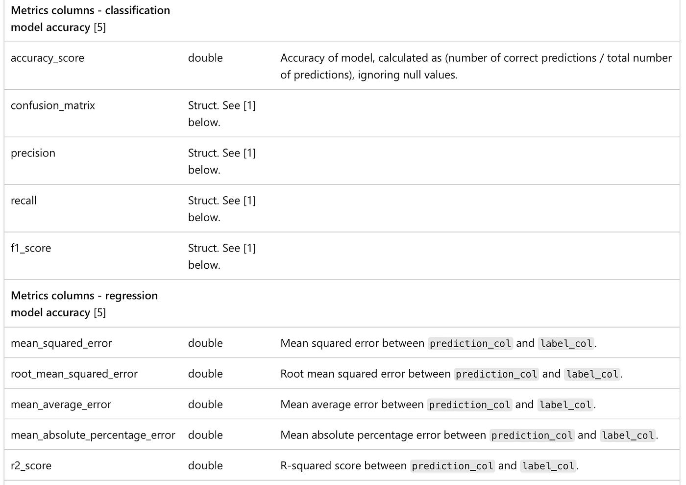
Profile Metrics Table
Stores summary stats for each feature in each time window (count, nulls, mean, stddev, min/max, etc.).
For inference logs: also tracks accuracy, confusion matrix, F1, MSE, R², and fairness metrics.
Supports slicing/grouping (e.g., by model ID or feature value).
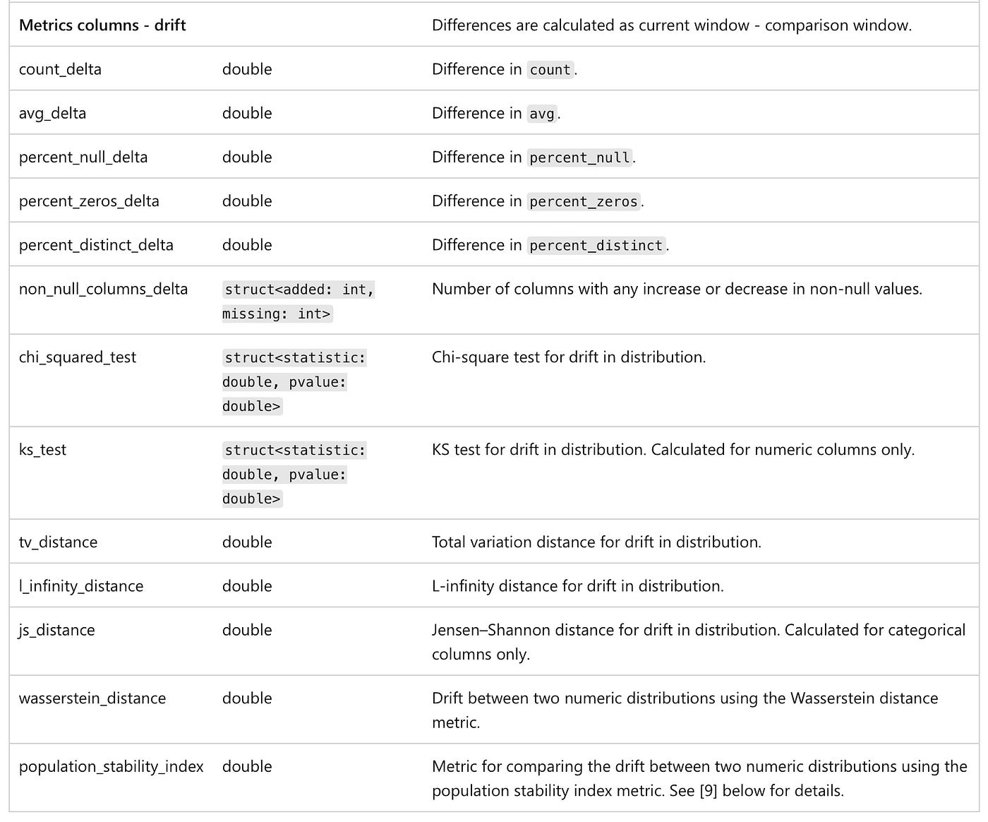
Drift Metrics Table
Tracks how your data’s column distributions evolve over time using advanced drift detection techniques
Essential for identifying data quality issues, detecting shifts in real-world behavior, and ensuring that model predictions remain reliable and unbiased.
There are two primary types of drift detection:
Consecutive Drift. Compares the current time window to the previous one to detect short-term anomalies or sudden changes.
Baseline Drift. Compares the current data to a fixed reference or baseline table, typically built from training data or a known “good” state.
Drift is calculated using a combination of statistical tests, distance metrics, and simple delta metrics. The table below shows which method work for which data type.
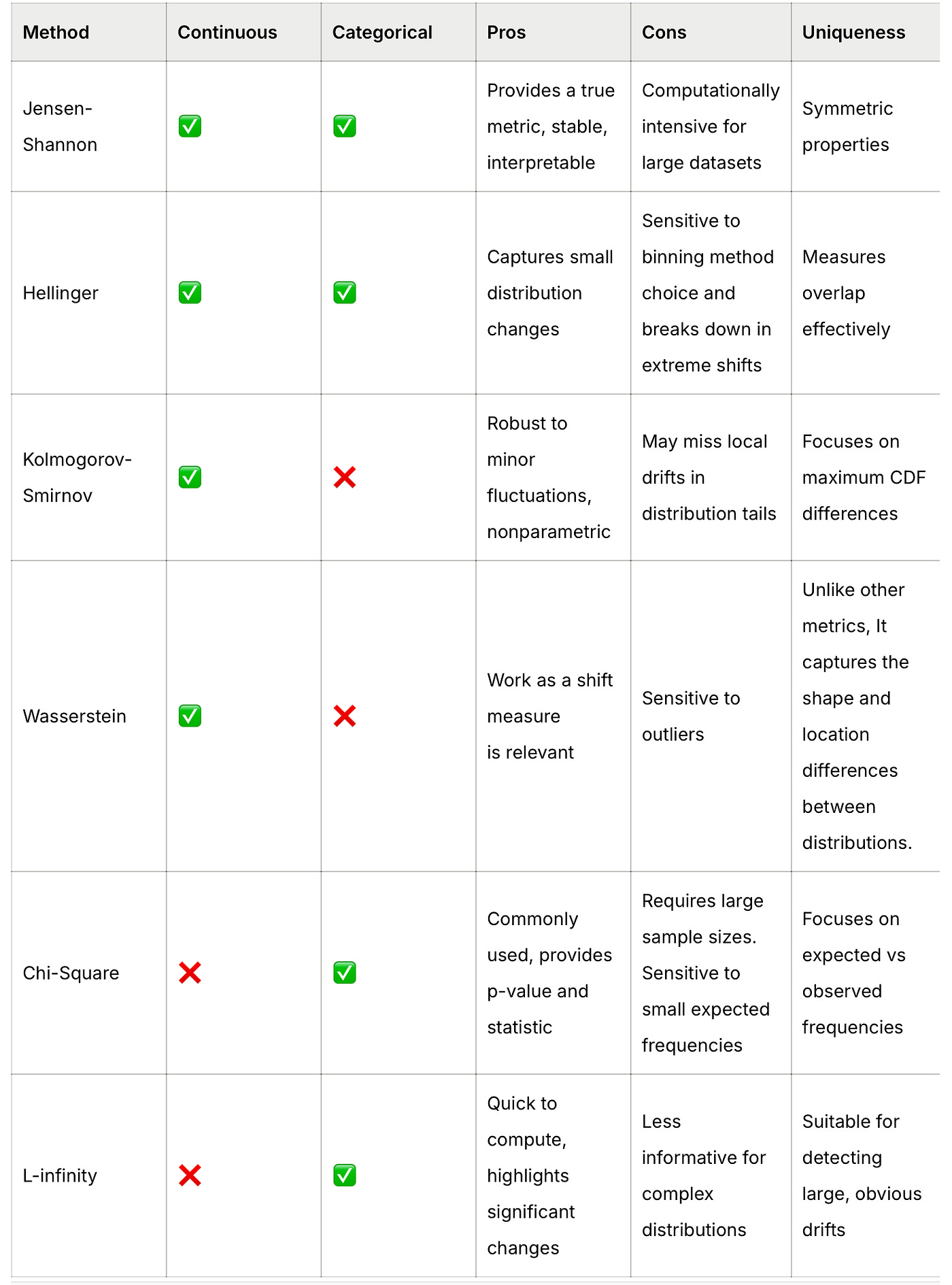
For detailed guidelines, you can check these articles: 1, 2. Also, the Little Book of Metrics is a great resource on ML model metrics.
Inference Tables
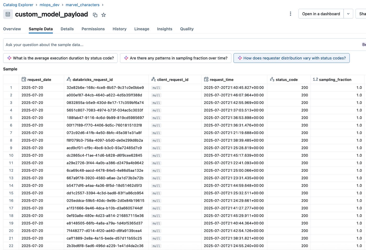
Inference tables are a built-in feature to log model inputs and predictions from a serving endpoint directly into a Delta table in Unity Catalog. This provides a simple way to monitor, debug, and optimize models in production.
Once enabled, they automatically capture request and response payloads, as well as metadata like response time and status codes etc. It’s used for:
Monitoring quality
Debugging
Training corpus generation
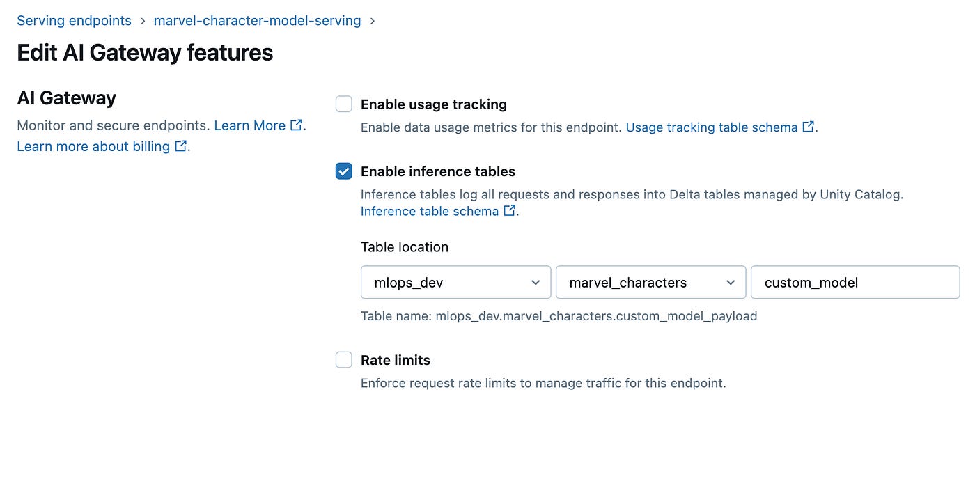
In order to create the inference table, you need to check enable inference table box when editing a serving endpoint (can also be created programmatically). The workspace must have Unity Catalog enabled, and you’ll need the right permissions to create and manage the associated Delta table.
Inference tables log raw data. To monitor drift/performance, process them into a structured inference profile table (with timestamp, features, prediction, and optionally ground truth).
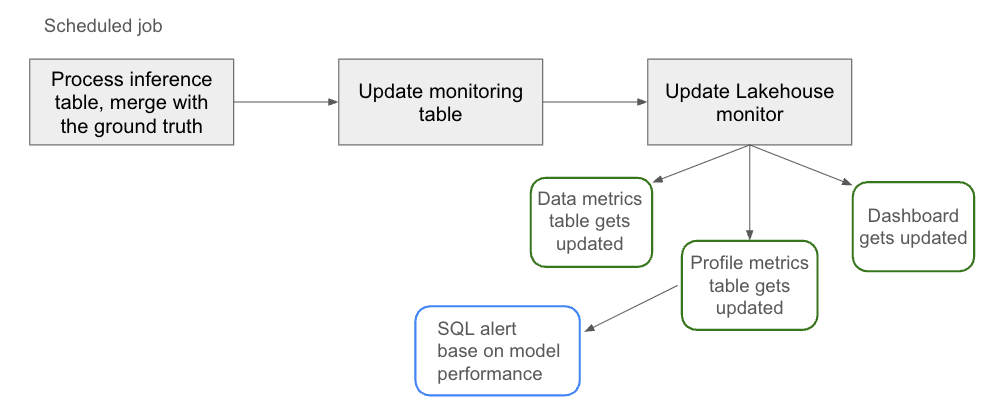
You can set up an automated job that processes the raw inference table into a structured monitoring table. This monitoring table would be used to
Update generate a metrics table
Automatically update the dashboard
You can also configure alerts, so you’re notified when performance drops or data shifts.
Monitoring pipeline
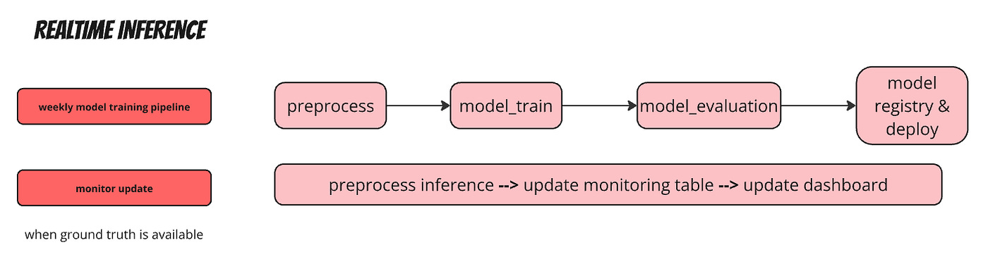
Let’s take a look at a model serving use case, similar to what we cover in the course. For example, there is a dynamic pricing model that gets retrained weekly, and the updated model is deployed to the serving endpoint. The workflow is similar to what we covered in Lecture 7.
A separate workflow would be required to update the Lakehouse monitor when ground truth labels arrive. We’ll go through it in our final lecture.
In the end, we’ll have two workflows, one for training and deployment, and the other one — for monitoring:
Conclusions
Here are some key takeaways from this lecture:
ML monitoring goes beyond system metrics, it includes data quality, drift, and model performance.
Databricks Lakehouse Monitoring provides built-in tools for tracking data and model health over time.
Not all data drift is bad — always check model performance before reacting.
Inference tables + monitoring pipelines enable end-to-end visibility and alerting in production.
In the next lecture, we’ll demonstrate how to create a Lakehouse monitor on Databricks, and deploy the monitoring pipeline.